J’ai voulu, rependre la main sur ma santé en analysant par moi même les indicateurs. On va voir ensemble comment le faire et quels sont les résultats.
Choisir son bracelet
Il existe des tonnes de bracelets de santé, mon choix s’est porté sur le Xiaomi Mi Band 3 et ce pour plusieurs raisons.
Premièrement car il est pas cher ! Pour seulement 30€, ce n’est pas un investissement risqué. Pour ce prix, vous n’aurez pas les dernières technologies, mais suffisament pour analyser. Il peut se connecter en bluetooth LE, mesurer les pas, mesurer le rythme cardiaque ainsi que le sommeil. Il propose également des fonctionnalité basique : montre (évidement), réveil, notifications. Cela n’envoie pas du rêve, mais permet de descendre le prix au plus bas et l’autonomie au plus haut, puisqu’il tient facilement 3 semaines.
Deuxièmement pour la sécurité de vos données. En effet, ce bracelet est bête, il ne peut qu’envoyer les données sur le téléphone. Le bracelet ne peut pas vous espionner à votre insu, il n’a pas de micro, ni de GPS. Sans wifi ou 3g, il ne peut pas se connecter directement à internet. A mon sens, sa taille, son poids ainsi que son autonomie sont des garants qu’aucun micro ou connexion internet ne tourne à votre insu dessus.
Ce bracelet est donc parfaitement inoffencif pour votre vie privée, il est obligé de se connecter à votre téléphone. L’application Xiaomi par contre, je ne lui fait pas confiance. Les données doivent bien partir chez Jinping… Qu’importe, il suffit de changer l’application, vous pouvez utiliser GadgetBridge, ainsi vos données reste chez vous.
GadgetBridge a aussi une fonctionnalité interressante, il est possible d’exporter les données directement dans un fichier sqlite3. C’est indispensable de vérifier que l’on puisse sortir les données de l’application avant de commencer à collecter.
import pandas as pd
import numpy as np
import sqlite3
import datetime
import matplotlib.pyplot as plt
import seaborn as sns
from matplotlib import cm
%matplotlib inline
sns.set(style="darkgrid")
conn = sqlite3.connect('Gadgetbridge_20190403-215000')
df = pd.read_sql_query("select * FROM MI_BAND_ACTIVITY_SAMPLE ", conn)
df = df.set_index(pd.to_datetime(df.TIMESTAMP, unit='s'))
df.drop(['TIMESTAMP', 'DEVICE_ID', 'USER_ID'], axis=1, inplace=True)
df.head(5)
| RAW_INTENSITY | STEPS | RAW_KIND | HEART_RATE | |
|---|---|---|---|---|
| TIMESTAMP | ||||
| 2018-11-30 20:13:00 | 22 | 0 | 80 | 255 |
| 2018-11-30 21:14:00 | 40 | 0 | 80 | 255 |
| 2018-11-30 21:14:41 | -1 | -1 | 1 | 0 |
| 2018-11-30 21:14:42 | -1 | -1 | 1 | -1 |
| 2018-11-30 21:14:43 | -1 | -1 | 1 | -1 |
Clean data
Replace -1 by 0
df.replace(-1, 0, inplace=True)
Apply definition to kind
def find_kind(i):
    if i in [1, 16, 17, 26, 50, 66, 98]: # Walk
        return 'WALK'
    elif i in [112, 121]: # NREM
        return 'NREM'
    elif i in [122]: # REM
        return 'REM'
    elif i in [80, 90, 96, 91, 99]: # SIT
        return 'SIT'
    else: # UNKNOWN
        return 'UNKNOWN'
df['KIND'] = df['RAW_KIND'].apply(find_kind)
df = df[df['KIND'] != 'UNKNOWN']
Clean heart rate
df['HEART_RATE'][:] = df['HEART_RATE'].apply(lambda x: x if x < 200 else np.nan)
df.interpolate(inplace=True)
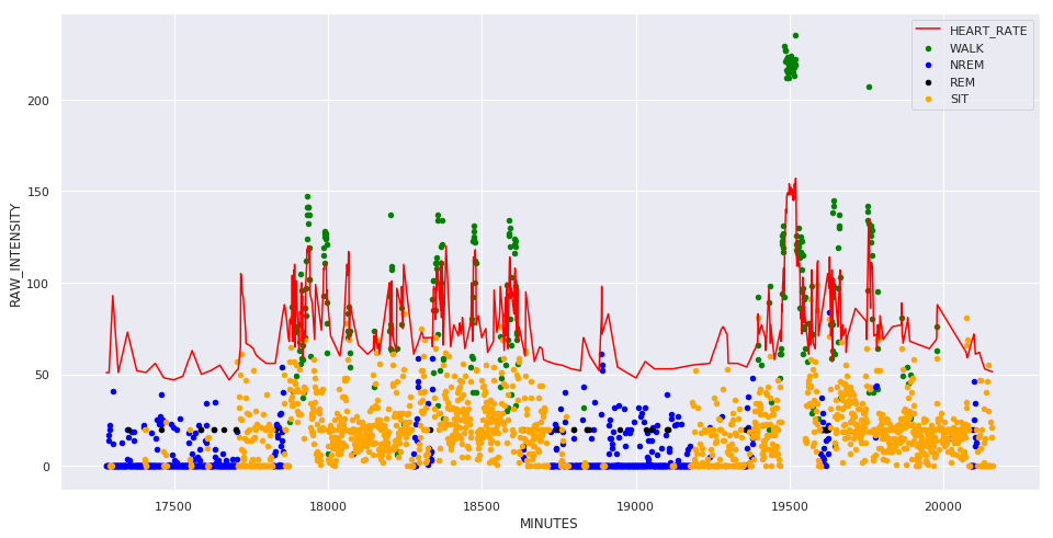
Display result
part = df.loc['2019-01-12':'2019-01-13']
part['MINUTES'] = part.index.day*1440 + part.index.hour*60 + part.index.minute
/home/francois/Projects/MiBand/venv/lib/python3.6/site-packages/ipykernel_launcher.py:2: SettingWithCopyWarning:
A value is trying to be set on a copy of a slice from a DataFrame.
Try using .loc[row_indexer,col_indexer] = value instead

See the caveats in the documentation: http://pandas.pydata.org/pandas-docs/stable/indexing.html#indexing-view-versus-copy
fig, ax = plt.subplots(figsize=(16, 8))
for kind, color in [['WALK', 'green'], ['NREM', 'blue'], ['REM', 'black'], ['SIT', 'orange']]:
    y = part[part['KIND'] == kind]
    y.plot.scatter('MINUTES', 'RAW_INTENSITY', color=color, label=kind, ax=ax)
ax.plot(part['MINUTES'], part['HEART_RATE'], color='red')
ax.legend()
plt.show()
Extract daily data
def count_steps(day, data):
    J1 = day + datetime.timedelta(days=1)
    return data[day:J1]['STEPS'].sum()
def count_activity_ratio(day, data):
    J1 = day + datetime.timedelta(days=1)
    d = data[day:J1]['KIND']
    w = d[d == 'WALK'].count()
    s = d[d == 'SIT'].count()
    return  w / (w + s)
def mean_heart_rate(day, data):
    J1 = day + datetime.timedelta(days=1)
    d = data[day:J1]['HEART_RATE']
    d = d[d > 30]
    return d.mean(), d.min(), d.max()
def count_sleep(today, data):
    # Get data from yesterday 20h to today 12h
    H19 = today - datetime.timedelta(hours=5)
    H14 = today + datetime.timedelta(hours=14)
    d = data[H19:H14]
    # print(H19, H14)

    # Select only timestamp a SIT kind with RAW_INTENSITY bigger than 25 over 10min
    d = d[d['KIND'] == 'SIT']['RAW_INTENSITY']
    d = d.resample('10T').mean().fillna(0)
    d = d > 20
    # print(d)

    # Find fall asleep
    try :
        H02 = today + datetime.timedelta(hours=2)
        start = d[d==True][H19:H02].index[-1]

        # Find wake up
        H06 = today + datetime.timedelta(hours=6)
        end = d[d==True][H06:H14].index[0]
        duration = end - start
        return start.hour+start.minute*60, end.hour+end.minute*60, duration.total_seconds() / 3600
    except IndexError:
        return np.nan, np.nan, np.nan
def build_row(today, data):
    steps = count_steps(today, data)
    activity = count_activity_ratio(today, data)
    heart_mean, heart_min, heart_max = mean_heart_rate(today, data)
    asleep, wakeup, sleep_time = count_sleep(today, data)

    return {'steps': steps, 'activity': activity,
            'heart_mean': heart_mean, 'heart_min': heart_min, 'heart_max': heart_max,
            'asleep': asleep, 'wakeup': wakeup, 'sleep_time': sleep_time}
start = df.index[0].replace(hour=0, minute=0) + datetime.timedelta(days=1)
end = df.index[-1].replace(hour=0, minute=0) - datetime.timedelta(days=1)
extract = pd.DataFrame(columns=['steps', 'activity', 'heart_mean', 'heart_min', 'heart_max', 'asleep', 'wakeup', 'sleep_time'], index=pd.date_range(start, end=end, freq='D'))
for date in extract.index:
    extract.loc[date] = build_row(date, df)
extract = extract.astype(float)
/home/francois/Projects/MiBand/venv/lib/python3.6/site-packages/ipykernel_launcher.py:6: RuntimeWarning: invalid value encountered in long_scalars
extract.dropna(inplace=True)
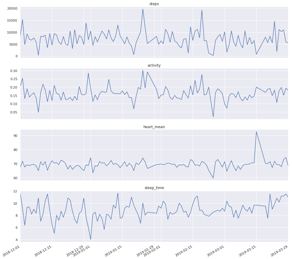
fig, ax = plt.subplots(nrows=4, ncols=1, figsize=(16, 16), sharex=True)
for a, col in zip(ax, ['steps', 'activity', 'heart_mean', 'sleep_time']):
    extract[col].plot(ax=a)
    a.set_title(col)
plt.show()
extract.head()
| steps | activity | heart_mean | heart_min | heart_max | asleep | wakeup | sleep_time | |
|---|---|---|---|---|---|---|---|---|
| 2018-12-01 | 8231.0 | 0.204225 | 67.314582 | 48.000000 | 122.0 | 621.0 | 3008.0 | 11.666667 |
| 2018-12-02 | 15249.0 | 0.253829 | 71.690354 | 30.923077 | 173.0 | 2421.0 | 3006.0 | 9.166667 |
| 2018-12-03 | 4809.0 | 0.130529 | 67.596080 | 30.130435 | 127.0 | 3023.0 | 606.0 | 6.333333 |
| 2018-12-04 | 9193.0 | 0.189886 | 69.228908 | 34.000000 | 117.0 | 2420.0 | 6.0 | 9.333333 |
| 2018-12-05 | 6999.0 | 0.139659 | 68.618289 | 47.000000 | 117.0 | 2420.0 | 6.0 | 9.333333 |
extract['weekday'] = extract.index.weekday
extract['monthday'] = extract.index.day
extract['month'] = extract.index.month
extract['week'] = extract.index.week
extract['weekend'] = extract['weekday'] > 5
def week_period(x):
    if 0 <= x < 2:
        return 'begining'
    elif 2 <= x <= 5:
        return 'middle'
    elif 5 < x:
        return 'weekend'
extract['week period'] = extract['weekday'].apply(week_period)
Analyze data
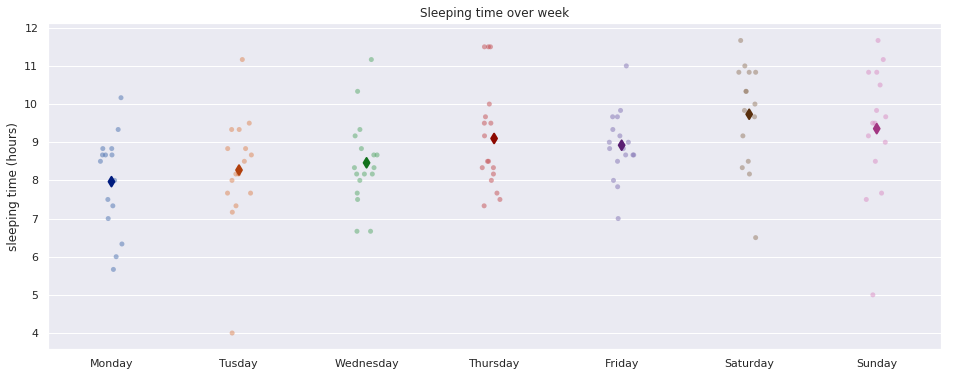
Sleep over the week
fig, ax = plt.subplots(figsize=(16,6))
sns.stripplot(x='weekday', y='sleep_time', data=extract, dodge=True, jitter=True, alpha=.5, zorder=1, ax=ax)
sns.pointplot(x='weekday', y='sleep_time', data=extract, dodge=0.532, join=False, palette='dark', markers='d', scale=1, ci=None,ax=ax)
ax.set_title('Sleeping time over week')
ax.set_xlabel('')
ax.set_xticklabels(['Monday', 'Tusday', 'Wednesday', 'Thursday', 'Friday', 'Saturday', 'Sunday'])
ax.set_ylabel('sleeping time (hours)')
plt.show()
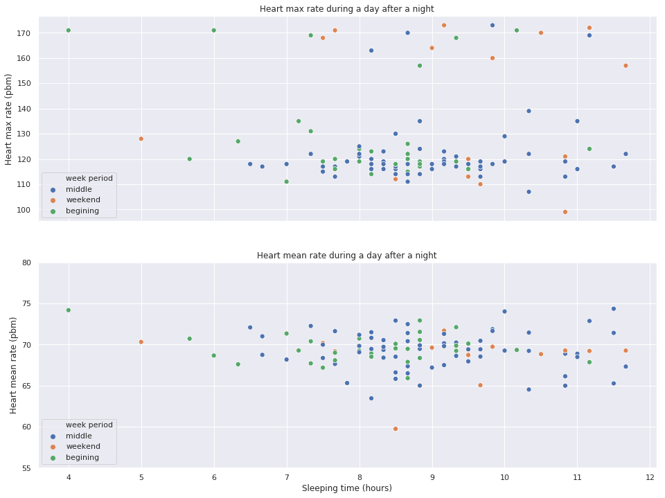
Day performance from last night sleep
fig, (top, bottom) = plt.subplots(nrows=2, figsize=(16, 12), sharex=True)
sns.scatterplot(x='sleep_time', y='heart_mean', alpha=1, data=extract, ax=bottom, hue='week period', s=50)
bottom.set_title('Heart mean rate during a day after a night')
bottom.set_ylabel('Heart mean rate (pbm)')
bottom.set_xlabel('Sleeping time (hours)')
bottom.set_ylim([55, 80])

sns.scatterplot(x='sleep_time', y='heart_max', alpha=1, data=extract, ax=top, hue='week period', s=50)
top.set_title('Heart max rate during a day after a night')
top.set_ylabel('Heart max rate (pbm)')

plt.show()
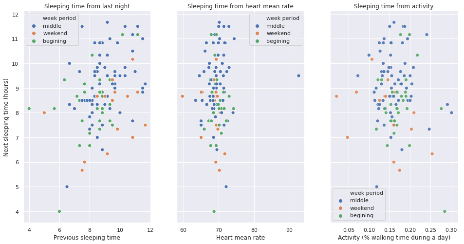
Next night sleep from day performance
extract['next_sleep_time'] = extract['sleep_time'].shift(periods=-1)
extract.drop(extract.index[-1], inplace=True)
fig, (left, middle, right) = plt.subplots(ncols=3, sharey=True, figsize=(16, 8))

sns.scatterplot(x='sleep_time', y='next_sleep_time', alpha=1, data=extract, hue='week period',ax=left, s=50)
left.set_title('Sleeping time from last night')
left.set_ylabel('Next sleeping time (hours)')
left.set_xlabel('Previous sleeping time')

sns.scatterplot(x='heart_mean', y='next_sleep_time', alpha=1, data=extract, hue='week period',ax=middle, s=50)
middle.set_title('Sleeping time from heart mean rate')
middle.set_ylabel('Next sleeping time (hours)')
middle.set_xlabel('Heart mean rate')

sns.scatterplot(x='activity', y='next_sleep_time', alpha=0.9, data=extract, hue='week period', ax=right, s=50)
right.set_title('Sleeping time from activity')
right.set_xlabel('Activity (% walking time during a day)')
plt.show()